

Programming in Two Dimensions
Wallace Feurzeig
BBN Systems and Technologies
70 Fawcett Street, Cambridge,
Massachusetts 01238, USA,
tel: 617-873-3448, fax: 617-873-2455,
email: feurzeig@bbn.com
Abstract
This paper describes Function Machines, a visual programming language for mathematics education, and illustrates its use in classroom applications. Functional programming languages are potentially powerful instruments for helping students develop mathematical ways of thinking. However, helping students acquire fluency in developing programs that are mathematically rich and compelling is a nontrivial task. Even Logo, the most accessible functional language, poses significant conceptual barriers to the acquisition of the requisite knowledge and skill. The principal ones are an understanding of the mechanisms for passing data and transferring control between procedures, particularly iterative and recursive control structures. Logo is often taught by teachers who are mathematically unskilled. Thus, elementary classroom work frequently comes to an intellectual impasse, dead-ending with kids drawing turtle pictures. Function Machines was expressly designed to overcome these barriers through the use of visual representations that make control structures and program operation greatly more accessible.
Keywords
Visual programming, mathematics, mathematics education, parallel processes, computer science
1 Introduction
Function Machines is a visual programming environment with the representational power of a universal programming language. It is based on a functional control structure and a dataflow model of program execution. Its key construct is the "function-machine", a visual isomorph of the function concept in mathematics. Machines are visual analogs of Logo procedures or Lisp functions. They communicate data to each other via "pipes" connecting the output of one to the input of another, in data-flow fashion. The sequence of execution between machines may be similarly directed by constructing "wires" connecting one machine to another. In the absence of such wiring, control flow among machines is unconstrained, and execution is essentially parallel.
The Function Machines language expresses program structures visually as two-dimensional graphic icons, in contrast with the symbolic textual expressions used in traditional (one-dimensional) languages. The system provides as primitive constructs, machines corresponding to the standard mathematical, graphics, list processing, logic, and I/O operations. These machines are used as building blocks to construct more complex machines in an extensible fashion. The explicit representation of data paths (by graphically animating the passage of data between machines) and of control paths (by illuminating currently active machines and by graphically animating the passage of control activation) makes the semantics of functional operation transparent in Function Machines in a fashion readily accessible to beginning students. Function Machines thus provides a natural starting point for a programming approach to the teaching of mathematics, and as a prelude and complement to nontrivial work with Logo.
2 Classroom Teaching Experiments
Function Machines supports a rich variety of mathematical explorations and investigations in elementary and secondary classrooms [1, 2, 3.] Its visual representations of program structures significantly aid in understanding computational processes. By explicitly showing the passage of data objects into and out of machines, and by illuminating the data and control paths as machines are run, computational processes are rendered as visual animations and the program semantics become a great deal more transparent.


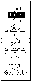
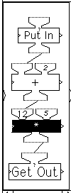
Figure 1 Stages in the operation of a four-machine calculation network.
The following sequence, part of a pre-algebra unit currently being used by students in fifth-grade math classes in US schools in Italy and Germany, illustrates the use and educational benefits of visual programming in Function Machines. Students begin by using the Function Machines program Predicting Results, an instance of which is shown in Figure 1.
Their task here is to guess what output will be produced by a given input. They run the machines to check out their guesses. Students enter a number in the Put In machine; it is printed on the display window shown on the right and it is also sent to the + machine, which adds 2 to it; the result is then sent to the * machine, which multiplies it by 5; that result is sent to the Get Out machine which prints it in the display window. The figure shows the successive stages in the computation across time. The machines that are active (ready to run) at any point in time are displayed in reverse video (black.) As the figure shows, an input of 10 generated an output of 60.
Using the same machine network, the students are challenged next, not to determine what output will be produced by a given input, as previously. Instead, their task is to determine an answer to the opposite question: what number must be input to produce a specified output? In this instance, using the +2 and *5 machines, what number must be Put In to Get Out 100?
Understandably, this seems to them a much more difficult problem. They are encouraged to approach the task by trial and error. The display screen on the right shows the results of a trial-and-error sequence aimed at finding what input yields an output of 100. The input 10 yields 60, so perhaps a larger input is needed. An input of 20 yields 110. So perhaps some input between 10 and 20 is called for. 15 yields 85; 17 yields 95, and then -- "Hooray! 18 works!" The sequence required five trials. Using the same pair of machines with other output targets, kids attempt to determine the correct inputs in as few trials as possible. They are delighted when they can zoom in on the answer in three or four trials and sometimes even two!
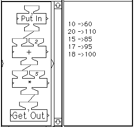
Figure 2 Inputs and outputs using the four-machine network.
In the Function Machines programming environment, a set of machines may be encapsulated under a single machine icon—a composite machine—which can then be used as a component of a more complex composite machine, or of itself. At this point, as shown in Figure 3, two composite machines, To Get Out and You Should Put In, are introduced to the students. The internal contents of these machines—the machines contained within them—are currently invisible.
The inputs and outputs produced by these new machines are shown in Figure 3 on the right half of the display screen.
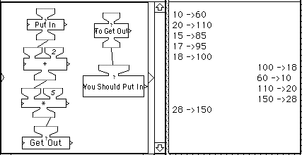
Figure 3 Working on the reverse prediction problem—how to generate a specified output.
Just after the last printout on the left was produced, showing that an input of 18 produces an output of 100, the two new machines are run. An input of 100, the target output in the previous problem, is given to the To Get Out machine. This input is piped to the You Should Put In machine which produces the printout of 18 shown on the display. Somehow, using this pair of machines, all one had to do was give it the desired output and it produced the corresponding input—and in just a single trial! Also, rest of the printout from this machine confirms what was shown before, that to get an output of 60 requires an input of 10, an output of 110 calls for an input of 20. And it could be used to confirm the other pairs also -- that an output of 85 calls for an input of 15, etc. Instead, however, it is used to assert a new claim, that to get an output of 150 requires an input of 28. The last printout on the left of the display, generated by running the four-machine network, confirms this, i.e., an input of 28 indeed yields an output of 150.

Figure 4 Inside the Reversing Machine.
The problem for the students is: how does the You Should Put In machine know, right from the start, what input one needs to put in to get a desired output? What kind of magic does it use? They are not expected to fathom the answer. Instead, they are shown the inner contents of the machine, seen here in Figure 4.
As the figure shows, the solution to the problem is to do the inverse computations in the opposite order. The original computation sequence was: put in a number (say N), add 2 to it, multiply the result by 5, and get out the answer. To undo this sequence, one computes operations in the reverse order from the original sequence, replacing the original operations with their inverses, as follows: put in the desired answer, divide it by 5, subtract 2 from the result and get out N. This is essentially the algorithm for solving linear equations in algebra, and in this interactive visual context, fifth-graders understand its sense and purpose.
3 Iteration and Recursion in Function Machines
The programs shown above, though educationally empowering, are at a low level of computational complexity. Iterative and recursive processes are essential for building more powerful programs but their use is often very difficult for beginning students. The dynamic visual dataflow representations of control structures in Function Machines facilitate students’ understanding and development of mathematically rich and computationally powerful processes. The simplest form of iteration, called backput iteration, is introduced on the students’ first day with Function Machines.
Figure 5 illustrates backput iteration with a primitive (built-in) machine and also with a composite (user-constructed) machine. The top of the leftmost frame shows a plus machine with two inputs, 0 and the constant 1.The output of this machine is piped back to the left input hopper. Thus, each time the plus machine runs, the new sum is output to the left hopper.

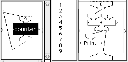
Figure 5 Backput iteration and the counting machine.
The bottom of the frame shows the plus machine after nine iterations, ready to run by adding the last output (9) to 1.The second frame shows backput iteration with a composite machine, called counter, whose inner contents (a plus machine and a print machine) are shown in the rightmost frame. Each time counter runs it adds 1 to its previous sum and prints the result to a display window, shown in the center frame.
Figure 6 shows the use of a built-in iteration machine, the Repeat machine. Each time a Repeat machine runs it decrements its first input (the number of iterations remaining) and carries out the computation called for in its inner body. In the example shown, the Repeat machine draws a turtle figure, a closed spiral, by repeating 100 times a left turn (initially 40 degrees, incremented each time by a constant of 30 degrees) and a constant forward step of 10 units.
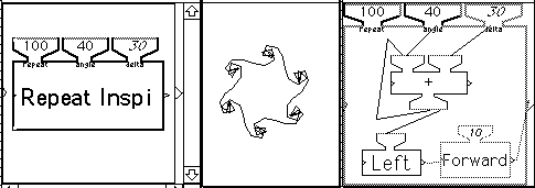
Figure 6 Using iteration with the Repeat machine to generate a closed spiral.
Function Machines includes primitive machines for more complex forms of iteration than that provided by the Repeat machine, including a For-loop machine, and a To-Each machine (which applys an iteration over a set of inputs.) Nested iterative operations are a great deal easier to follow in this iconic visual form than in the usual one-dimensional textual representation.
Even more striking in its clarity is the.Function Machines representation of recursion. Recursion is a great deal more confusing than iteration to beginning students. The idea of a procedure being defined in terms of itself seems cryptic, circular, even nonsensical. The sense and operation of recursion becomes marvelously clear in Function Machines, opening the way for students to experience and explore the extraordinary mathematical power of recursive processes. Figure 7 shows the use of recursion in a Function Machines program, the polyspi machine.

Figure 7 Recursive computation of a polygonal spiral.
The inner body of polyspi is shown on the right. Each time polyspi runs, the turtle moves forward 10 units and turns right (117 degrees initially, incremented by 3 degrees on each new call of polyspi.) The inclusion of the polyspi machine icon inside its own inner body is accomplished in a straightforward way. First polyspi is saved in unfinished form (without the polyspi machine icon in its body.) This causes the icon to be included in the composite machine menu. Then polyspi is retrieved and the polyspi icon is copied from the menu into the body of the machine.
Figure 8 shows the combined use of recursion and iteration. The inner body of the Triangles machine is an iterative Repeat machine (not shown) whose inner body is shown on the right. The repeat machine is run three times. Each time it runs it calls the Triangles machine recursively.

Figure 8 Combining iteration and recursion to generate a Sierpinski triangle.
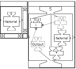
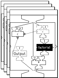
Figure 9 The factorial machine: outside and inside views.
The operation of recursion is made visually explicit by displaying a separate window for each instantiation of the procedure as it is created, and erasing it when it terminates. Figure 9 shows how recursive processes are presented when these windows are displayed during a run. The figure shows in the left frame a composite machine (factorial) for computing the factorial function recursively. When a composite machine fires it can be set to automatically x-ray. This has the effect of opening a new window with the contents of the composite displayed. The various components of the composite fire as the program executes. In turn, if any of the components are composites they too can automatically x-ray, opening a new window showing their components and the program will display the execution in that window.
The structure of the factorial composite factorial machine is displayed in this x-ray view. Factorial contains four primitive machines: the less-than-or-equal machine (<) , the Output machine, the subtraction machine (-), and the multiplication machine (*) It also contains a copy of itself. The computational logic is straightforward. The factorial machine takes as input a positive integer n. It passes n to three hoppers, the left hopper of the < machine, the left hopper of the - machine, and the left hopper of the * machine. It tests to see if n is less than 2. If so, it outputs 1 and the process is done. If not, it subtracts 1 from n and computes the factorial of that number (n-1). After it obtains the result—the factorial of (n-1)—it multiplies that by n and outputs the product.
The middle frame in Figure 9 shows the initial x-ray window, corresponding to factorial of 5. When factorial of 5 is run it calls for factorial of 4, which calls for factorial of 3, and so on. The frame on the right shows the stack of windows generated during the run, corresponding to successive x-rays of the factorial machine for factorial of 5 (whose x-ray window is on the bottom of the stack), then factorial 4, factorial 3, and factorial 2 (the top window.) At this point, the program is about to compute factorial of 1. The factorial 1 machine outputs its result, 1, to the factorial 2 machine, after closing its window and thus exposing the window of the factorial 2 machine. This machine can now ouput its result, 2, to the factorial 3 machine after closing its window and exposing the window of the factorial 3 machine. In turn, the factorial 3 machine outputs its result, 6, to the factorial 4 machine. And so on until, finally, the factorial 5 machine computes its result, closes its x-ray window, and passes the result to the output hopper of the parent machine, shown in the left frame.
Operating in this fashion, the Function Machines device of creating an x-ray window for each instance of a composite call provides a clear and concrete dynamic visual model of the recursive computational process.
4 Parallel Computation
In the Function Machines environment, a machine runs whenever its inputs are available. Since this can occur simultaneously for several machines, the system naturally supports concurrency and parallel computation. Thus, as well as its unique and valuable potential as a starting programming language for beginning students, Function Machines opens opportunities for introducing very early the advanced subject of parallel algorithms and models.
An example of such a multi-turtle simulation is the classic "turtle tag" problem: to describe the pattern generated by the tracks of four turtles, initially postitioned at the vertices of a square, each simultaneously moving counterclockwise toward its nearest neighbor. Figure 10 shows a Function Machines model of the turtle tag dance.
The turtle display (in the right window) shows the initial positions of the turtles. As the program runs, each turtle first computes the heading of its nearest neighbor. Thus, turtle a seeks turtle d, d seeks c, c seeks b, and b seeks a. Then, each turtle moves a short distance along its new heading and the process continues with further rounds of seeks and moves. The output of each Move machine passes the current position and heading of its turtle to the appropriate Seek machine to ready it for its next computation. Figure 10 shows the Turtle Tag program in operation. As the left window shows, the four Seek machines are ready to run. Note that all four have been activated at the same time so they will run concurrently. The program has been in operation for some time. The right window shows the tracks that have been generated thus far.
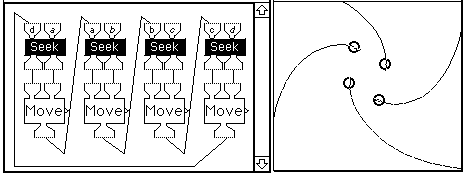
Figure 10 On the way.
Figure 11 shows the turtles' final position. It illustrates the use of simultaneous visualizations of the program structure and operation, as well as its output behavior.
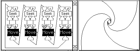
Figure 11 Rendezvous.
As the program runs, one can see the processes that are currently computing. At the same time one also sees what effects these processes have on the model's visual outputs. Moreover, one can study the relation between the program description and the program output more intensively by running the program incrementally, one step at a time. Observing the dynamic visualization of the model processes can give students very direct insight into the mechanisms underlying the model's visual outputs. The benefits from working with both kinds of visualizations increase as models become more complex.
The Function Machines program was originally implemented in 1989. It runs on all Macintosh systems. We are currently working on a Java-based implementation with the goal of enhancing its functionality, interface, and performance. It will run on Windows machines as well as Macintosh platforms.
References